Data Warehouse 101 - Part 1

Two pioneers of data warehousing named Bill Inmon and Ralph Kimball had different approaches to data warehouse design.

Kimball Method:

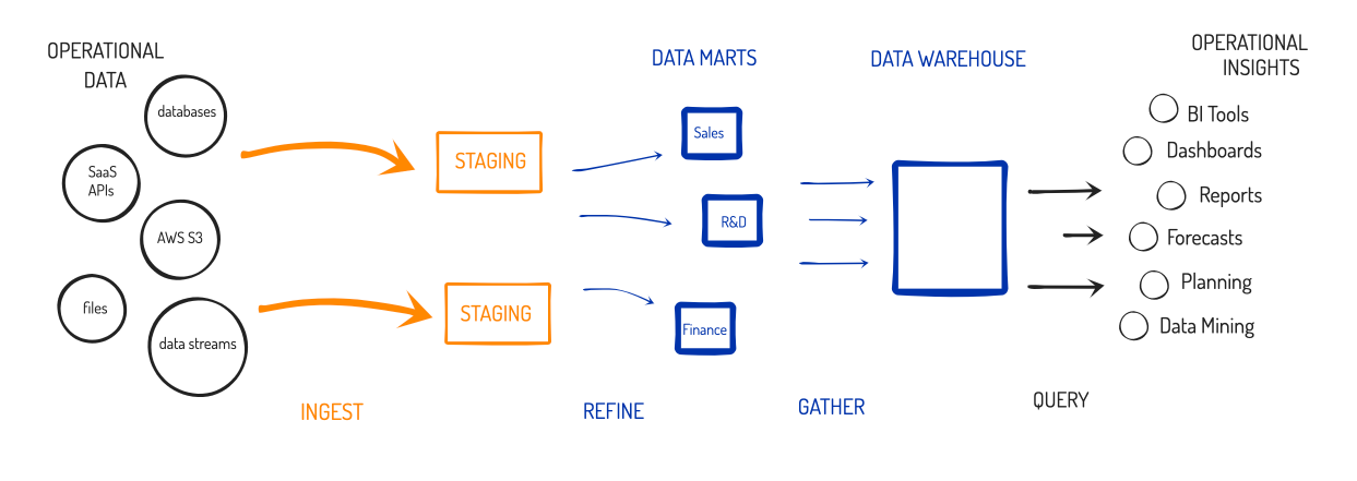
Build Data Marts for each line of Business with refine data and then Load to Data Warehouse.The Kimball data warehouse design uses a “bottom-up” approach.

Inmon Method:

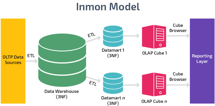
Build Data warehouse with refined data and then build Data Marts for each line of Business/Subject area.This is known as a top-down approach to data warehousing

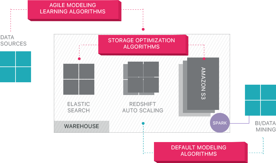
Data Warehouse Architecture: Traditional vs. Cloud

A data warehouse is an electronic system that gathers data from a wide range of sources within a company and uses the data to support management decision-making.

Companies are increasingly moving towards cloud-based data warehouses instead of traditional on-premise systems. Cloud-based data warehouses differ from traditional warehouses in the following ways:

• There is no need to purchase physical hardware.
• It’s quicker and cheaper to set up and scale cloud data warehouses.
• Cloud-based data warehouse architectures can typically perform complex analytical queries much faster because they use massively parallel processing (MPP).

The rest of this article covers traditional data warehouse architecture and introduces some architectural ideas and concepts used by the most popular cloud-based data warehouse services.

For more details, see our page about data warehouse concepts in this guide.

Traditional Data Warehouse Architecture

The following concepts highlight some of the established ideas and design principles used for building traditional data warehouses.

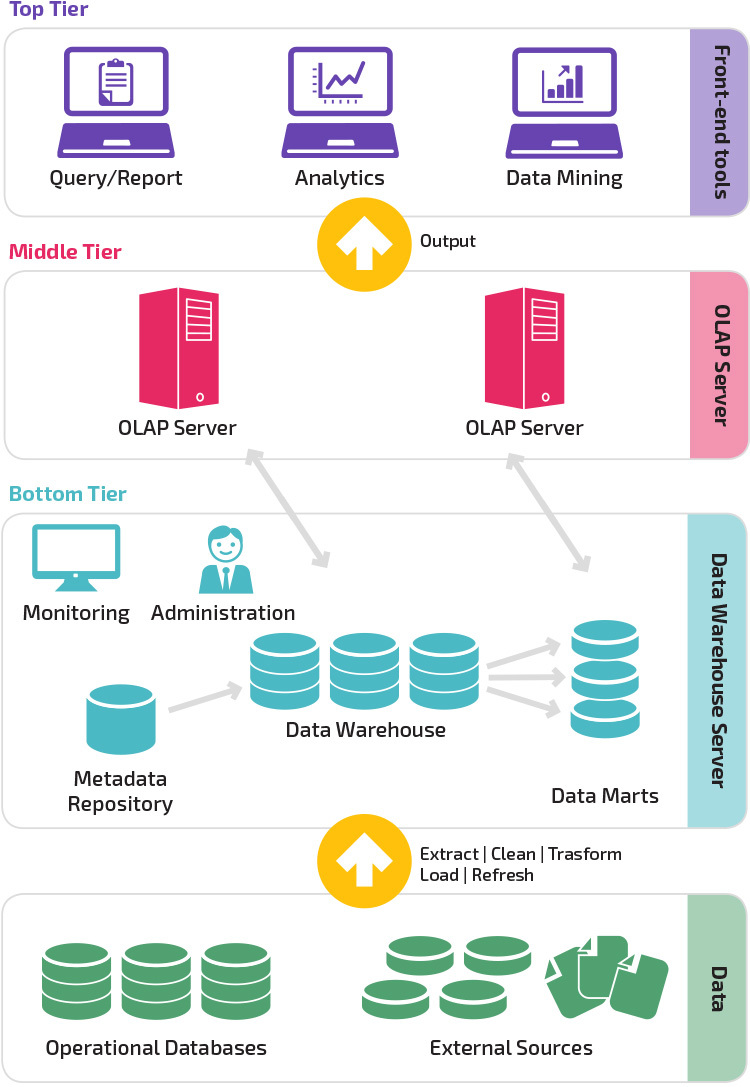
Three-Tier Architecture

Traditional data warehouse architecture employs a three-tier structure composed of the following tiers.

• Bottom tier: This tier contains the database server used to extract data from many different sources, such as from transactional databases used for front-end applications.
• Middle tier: The middle tier houses an OLAP server, which transforms the data into a structure better suited for analysis and complex querying. The OLAP server can work in two ways: either as an extended relational database management system that maps the operations on multidimensional data to standard relational operations (Relational OLAP), or using a multidimensional OLAP model that directly implements the multidimensional data and operations.
• Top tier: The top tier is the client layer. This tier holds the tools used for high-level data analysis, querying reporting, and data mining.

Kimball vs. Inmon

Two pioneers of data warehousing named Bill Inmon and Ralph Kimball had different approaches to data warehouse design.

Ralph Kimball’s approach stressed the importance of data marts, which are repositories of data belonging to particular lines of business. The data warehouse is simply a combination of different data marts that facilitates reporting and analysis. The Kimball data warehouse design uses a “bottom-up” approach.

Bill Inmon regarded the data warehouse as the centralized repository for all enterprise data. In this approach, an organization first creates a normalized data warehouse model. Dimensional data marts are then created based on the warehouse model. This is known as a top-down approach to data warehousing.

Data Warehouse Models

In a traditional architecture there are three common data warehouse models: virtual warehouse, data mart, and enterprise data warehouse:

• A virtual data warehouse is a set of separate databases, which can be queried together, so a user can effectively access all the data as if it was stored in one data warehouse.
• A data mart model is used for business-line specific reporting and analysis. In this data warehouse model, data is aggregated from a range of source systems relevant to a specific business area, such as sales or finance.
• An enterprise data warehouse model prescribes that the data warehouse contain aggregated data that spans the entire organization. This model sees the data warehouse as the heart of the enterprise’s information system, with integrated data from all business units.

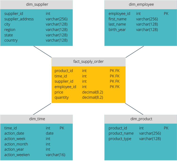
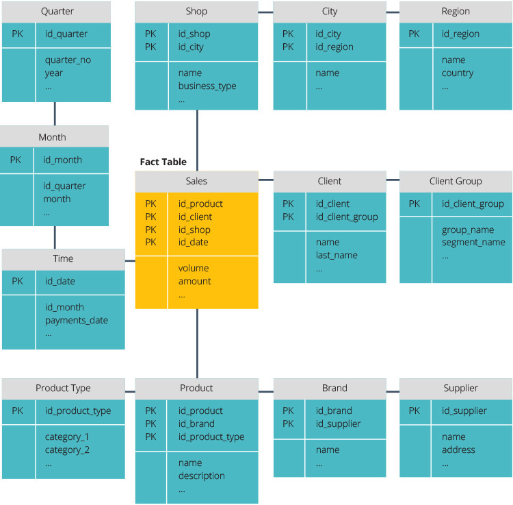
Star Schema vs. Snowflake Schema

The star schema and snowflake schema are two ways to structure a data warehouse.

The star schema has a centralized data repository, stored in a fact table. The schema splits the fact table into a series of denormalized dimension tables. The fact table contains aggregated data to be used for reporting purposes while the dimension table describes the stored data.

Denormalized designs are less complex because the data is grouped. The fact table uses only one link to join to each dimension table. The star schema’s simpler design makes it much easier to write complex queries.

The snowflake schema is different because it normalizes the data. Normalization means efficiently organizing the data so that all data dependencies are defined, and each table contains minimal redundancies. Single dimension tables thus branch out into separate dimension tables.

The snowflake schema uses less disk space and better preserves data integrity. The main disadvantage is the complexity of queries required to access data—each query must dig deep to get to the relevant data because there are multiple joins.

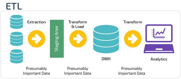
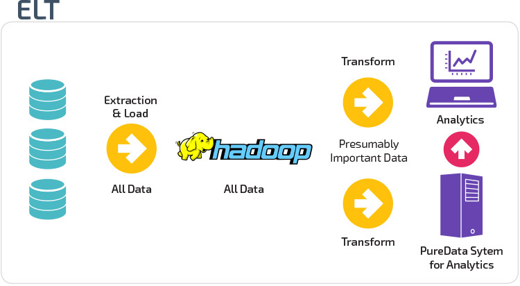
ETL vs. ELT

ETL and ELT are two different methods of loading data into a warehouse.

Extract, Transform, Load (ETL) first extracts the data from a pool of data sources, which are typically transactional databases. The data is held in a temporary staging database. Transformation operations are then performed, to structure and convert the data into a suitable form for the target data warehouse system. The structured data is then loaded into the warehouse, ready for analysis.

With Extract Load Transform (ELT), data is immediately loaded after being extracted from the source data pools. There is no staging database, meaning the data is immediately loaded into the single, centralized repository. The data is transformed inside the data warehouse system for use with business intelligence tools and analytics.

Organizational Maturity

The structure of an organization’s data warehouse also depends on its current situation and needs.

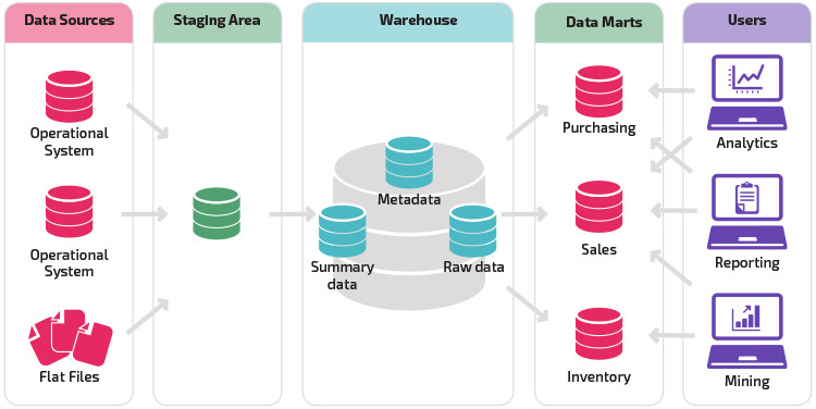
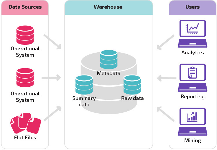
The basic structure lets end users of the warehouse directly access summary data derived from source systems and perform analysis, reporting, and mining on that data. This structure is useful for when data sources derive from the same types of database systems.

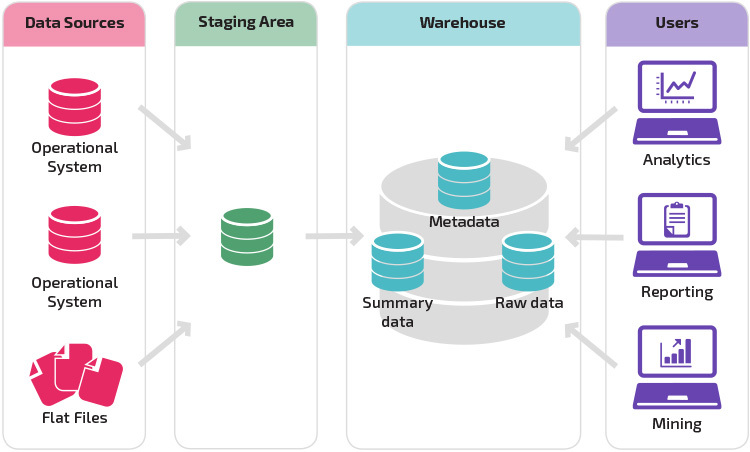
A warehouse with a staging area is the next logical step in an organization with disparate data sources with many different types and formats of data. The staging area converts the data into a summarized structured format that is easier to query with analysis and reporting tools.

A variation on the staging structure is the addition of data marts to the data warehouse. The data marts store summarized data for a particular line of business, making that data easily accessible for specific forms of analysis. For example, adding data marts can allow a financial analyst to more easily perform detailed queries on sales data, to make predictions about customer behavior. Data marts make analysis easier by tailoring data specifically to meet the needs of the end user.

New Data Warehouse Architectures

In recent years, data warehouses are moving to the cloud. The new cloud-based data warehouses do not adhere to the traditional architecture; each data warehouse offering has a unique architecture.

This section summarizes the architectures used by two of the most popular cloud-based warehouses: Amazon Redshift and Google BigQuery.

Amazon Redshift

Amazon Redshift is a cloud-based representation of a traditional data warehouse.

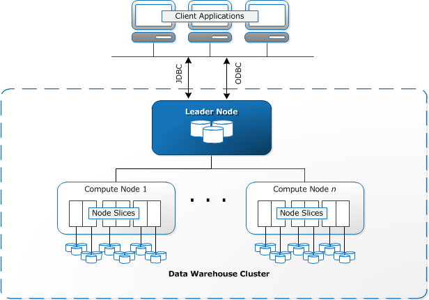
Redshift requires computing resources to be provisioned and set up in the form of clusters, which contain a collection of one or more nodes. Each node has its own CPU, storage, and RAM. A leader node compiles queries and transfers them to compute nodes, which execute the queries.

On each node, data is stored in chunks, called slices. Redshift uses a columnar storage, meaning each block of data contains values from a single column across a number of rows, instead of a single row with values from multiple columns.

Source: AWS Documentation

Redshift uses an MPP architecture, breaking up large data sets into chunks which are assigned to slices within each node. Queries perform faster because the compute nodes process queries in each slice simultaneously. The Leader Node aggregates the results and returns them to the client application.

Client applications, such as BI and analytics tools, can directly connect to Redshift using open source PostgreSQL JDBC and ODBC drivers. Analysts can thus perform their tasks directly on the Redshift data.

Redshift can load only structured data. It is possible to load data to Redshift using pre-integrated systems including Amazon S3 and DynamoDB, by pushing data from any on-premise host with SSH connectivity, or by integrating other data sources using the Redshift API.

Google BigQuery

BigQuery’s architecture is serverless, meaning Google dynamically manages the allocation of machine resources. All resource management decisions are, therefore, hidden from the user.

BigQuery lets clients load data from Google Cloud Storage and other readable data sources. The alternative option is to stream data, which allows developers to add data to the data warehouse in real-time, row-by-row, as it becomes available.

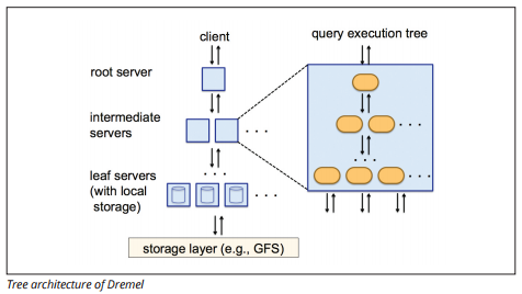
BigQuery uses a query execution engine named Dremel, which can scan billions of rows of data in just a few seconds. Dremel uses massively parallel querying to scan data in the underlying Colossus file management system. Colossus distributes files into chunks of 64 megabytes among many computing resources named nodes, which are grouped into clusters.

Dremel uses a columnar data structure, similar to Redshift. A tree architecture dispatches queries among thousands of machines in seconds.

Image source

Simple SQL commands are used to perform queries on data.

Panoply

Panoply provides end-to-end data management-as-a-service. Its unique self-optimizing architecture utilizes machine learning and natural language processing (NLP) to model and streamline the data journey from source to analysis, reducing the time from data to value as close as possible to none.

Panoply’s smart data infrastructure includes the following features:

• Analyzing of queries and data – identifying the best configuration for each use case, adjusting it over time, and building indexes, sortkeys, diskeys, data types, vacuuming, and partitioning.
• Identifying queries that do not follow best practices – such as those that include nested loops or implicit casting – and rewrites them to an equivalent query requiring a fraction of the runtime or resources.
• Optimizing server configurations over time based on query patterns and by learning which server setup works best. The platform switches server types seamlessly and measures the resulting performance.

Beyond Cloud Data Warehouses

Cloud-based data warehouses are a big step forward from traditional architectures. However, users still face several challenges when setting them up:

• Loading data to cloud data warehouses is non-trivial, and for large-scale data pipelines, it requires setting up, testing, and maintaining an ETL process. This part of the process is typically done with third-party tools.
• Updates, upserts, and deletions can be tricky and must be done carefully to prevent degradation in query performance.
• Semi-structured data is difficult to deal with - needs to be normalized into a relational database format, which requires automation for large data streams.
• Nested structures are typically not supported in cloud data warehouses. You will need to flatten nested tables into a format the data warehouse can understand.
• Optimizing your cluster—there are different options for setting up a Redshift cluster to run your workloads. Different workloads, data sets, or even different types of queries might require a different setup. To stay optimal you’ll need to continually revisit and tweak your setup.
• Query optimization—user queries may not follow best practices, and consequently will take much longer to run. You may find yourselves working with users or automated client applications to optimize queries so that the data warehouse can perform as expected.
• Backup and recovery—while the data warehouse vendors provide numerous options for backing up your data, they are not trivial to set up and require monitoring and close attention.